Methods How each of the seven methods is built, with code
Pick a paper to see why it was proposed, how its pipeline works step by step, what its circuit looks like, and runnable code in Python, Qiskit or PennyLane.
Library The seven papers, readable here
Pick a paper to open it in the viewer below, or open it in its own tab.
Try it Run the methods on your own graph
Load a built-in network (including three temporal benchmark topologies from Paper 1) or drop your own edge list, and all 11 classical and quantum methods below score the exact same held-out links. All four quantum paradigms—Projected Quantum Kernel (Paper 2/5), Variational Quantum Circuit (Paper 4), Data Re-Uploading QNN (Paper 6), and Continuous-Time Quantum Walk (Paper 3)—run as exact statevector simulations in your browser. Uploaded files never leave your device.
Choose a network
Pick a built-in network or upload your own edge list. With a third timestamp column the split is temporal and the timeline below switches on.
u v or u v timestamp (spaces, tabs or commas; lines starting with # are skipped; .gz works). For example, SNAP's CollegeMsg.txt.gz from snap.stanford.edu loads as-is.Classical vs quantum, same test links
ROC curves for every scorer. Click a row to hide or show its curve. Quantum curves are drawn thicker.
Timeline playback
The network is cut into 8 time steps. At each step the chosen method predicts the next links from the past only. Then you see which ones actually formed.
Circuit inspector
The exact 4-qubit circuit for one node pair. Pick any row above with Inspect circuit, then export it to Qiskit or OpenQASM and run the same circuit on IBM Quantum.
Playground What changes a prediction? Quantum and classical models side by side
Change the graph and time features, or load one of the example scenarios, and watch how each model's score moves: classical heuristics, a random forest, a variational circuit (P(q_0=1)), a quantum kernel SVM and the simple persistence baseline.
1. Preset graph topology
2. Interactive topological parameters
Live prediction probability output
Comparison The seven papers side by side
One row per paper. The columns follow the pipeline from left to right: qubits, the graph features that go in, how they are compressed, the circuit that encodes them, what is measured, and the classical model that makes the final call. The last column summarises what our reproduction found.
| Paper & Citation | Qubits (q) | Classical Features Extracted (D) | Compression / Prep Method | Quantum Encoding & Circuit Ansatz | Quantum vs Classical Classifier | Measurement Readout | Key Datasets | Benchmarking & Audit Findings | Read Paper PDF |
|---|---|---|---|---|---|---|---|---|---|
| Paper 1: QLP Manuscript Draft (Thakur, Mishra, Parihar, 2026 — 60p) |
q = 4, 6 | All feature families: local (CN, JC, AA, RA, PA), global (SP, LP, L3, CCLP), random walks (DeepWalk, node2vec, Walklets, CTDNE), GNNs (GCN, GraphSAGE, GAT) and repeat-edge baselines. | StandardScaler and PCA fitted on Strain only (ℝ24 → ℝ6 and ℝ16 / ℝ36 → ℝ4). Classical comparators receive exactly the same compressed features. | Reproduces & stress-tests PQKLP (ZZFeatureMap) & PQCLP (ZZFeatureMap + RealAmplitudes / EfficientSU2). | Matched comparisons: each quantum variant against a classical model on the same data, splits and features. | 1-RDM Pauli projections & Qubit-0 P(q0=1) = 1 − ⟨Z0⟩2. | Five temporal networks: MIT, Radoslaw-email, Eu-core, fb-forum and CollegeMsg. | Re-runs every method under one protocol. The persistence control (SeenBefore) reaches 0.93–0.99 AUC on four of five networks, and no snapshot-based quantum method beats the strongest classical configuration on any of them. | Open PDF (60p) |
| Paper 2: PQKLP (Kumar, Mishra, Biswas, 2022) |
q = 6 | 6 topological indices (CN, JC, AA, RA, PA, SP) across 4 snapshots G1..G4 = 24D. | StandardScaler + PCA reduction (ℝ24 → ℝ6). | ZZFeatureMap UΦ(z): Hadamard H⊗6 followed by pairwise (π−zk)(π−zm)ZkZm couplings. No trainable quantum weights. | Projected Quantum Kernel SVM vs Classical RBF-SVM & Random Forest. | Single-qubit reduced density matrices ρk(e) = Trj≠k[ρ(e)], read out as Pauli ⟨Xk⟩, ⟨Yk⟩, ⟨Zk⟩. | radoslaw-email, email-Eu-core, CollegeMsg | Projecting to single-qubit states avoids the kernel concentration of full-state fidelity. Under our protocol its best AUC was 0.85–0.98, below the strongest classical model on all five networks. | Open PDF |
| Paper 3: QLPCN / QLP (Moutinho et al., 2023) |
N Qubits (or log-space walk) + 1 Ancilla | The adjacency matrix itself, A ∈ {0, 1}N × N. No hand-built features and no PCA. | Node subspace initialization + 1 Ancilla Qubit |a⟩ = |0⟩ + eiφ|1⟩√2. | Continuous-time quantum walk (CTQW) U(t) = exp(−iAt), controlled by an ancilla qubit. | Quantum Transition Probability Ranking vs Classical Katz Index, PageRank, & SimRank. | Measuring the ancilla separates even walks, cos(At), which count 2-hop paths like CN, from odd walks, sin(At), which count 3-hop paths like L3. | Social networks (triadic closure) & Biological Protein-Protein Interaction (PPI) networks. | Even walks score higher on social networks and odd walks on bipartite and protein networks. This was the claim that reproduced most closely in our study. | Open PDF |
| Paper 4: PQCLP (Singh, Kumar, Biswas, 2024) |
q = 4 | Three feature sets over G1..G4: • Local: 4×4 = 16 features (CN, JC, AA, RA) • Global: 4×4 = 16 features (SP, LP, L3, CCLP) • Combined: 9×4 = 36 features |
StandardScaler + PCA reduction (ℝ16 / ℝ36 → ℝ4). | A data-encoding map (Z or ZZFeatureMap) followed by a trainable ansatz V(θ): RealAmplitudes (RY + CNOT) or EfficientSU2 (U3 + CNOT). | A variational circuit trained as the classifier with a BCE loss, compared with a random forest and an MLP. | Computational basis measurement strictly on Qubit 0: p̂θ(e) = P(q0=1) = 1 − ⟨Z0⟩2. | radoslaw-email, email-Eu-core, ia-contacts | The first end-to-end variational classifier for dynamic links. In our runs SPSA barely moved the weights from their initial values; with the same budget COBYLA raised the seed-1 test AUC to 0.62–0.80. | Open PDF |
| Paper 5: PQKELP (Kumar, Singh, Biswas, 2025) |
q = 5 | Random-walk node embeddings at several scales (DeepWalk, node2vec, Walklets), combined per pair with the Hadamard product hj(u,v) = zu ⊙ zv across G1..G4 (128 to 256 dimensions). | StandardScaler + PCA (→ 5D) + bounded scaling zk = π tanh(z̃k). | 5-Qubit IQP / ZZ-entangling quantum feature map UΦ(z(e)). | Projected quantum kernel embedding with an SVM or MLP, compared with node2vec and a random forest. | The full Bloch vector of every qubit, r(e) ∈ ℝ3q = ℝ15 (⟨Xk⟩, ⟨Yk⟩, ⟨Zk⟩). | Dynamic interaction networks, social communication graphs. | Random walks reach beyond the immediate neighbourhood, so pairs with no common neighbours still get a signal. Best AUC under our protocol was 0.76–0.87. | Open PDF |
| Paper 6: QGCNLP (Singh, Kumar, Sharma, Biswas, 2026) |
q = 4 | Node attribute matrices propagated through 2-layer Classical GCN: H(l+1) = σ(D̃−1/2 Ã D̃−1/2 H(l) W(l)). | Each node's aggregated GCN representation h, mapped to rotation angles RY(π tanh(W h)) on q = 4 or 8 qubits. | Angle Encoding RY(zk) + Variational Quantum Circuit V(θ) with CNOT ring entanglement. | A hybrid quantum–classical network trained end to end with Adam and backpropagation through the simulated circuit. | Pauli-Z expectations of every qubit, [⟨Z1⟩, …, ⟨Zq⟩]⊤, added back to the node representation; pairs are scored with a cosine decoder. | Cora, Citeseer, dynamic citation & collaboration graphs. | Gradients flow through both the classical and quantum parts. Message passing must use training edges only: when we restricted it, every model's AUC dropped by 0.010 to 0.147. | Open PDF |
| Paper 7: A2QTGN (Innan et al., 2026) |
q = 4 | A stream of timestamped events (u, v, t) processed by TGN memory su(t) (a GRU) and temporal graph attention. | Learnable adaptive weighting α ⊙ huv(t) + L2-norm normalization into 2q = 16 normalized amplitudes. | Adaptive amplitude encoding of a 256-dimensional vector into q = 8 qubits (28 = 256 amplitudes), followed by one CNOT chain. The circuit itself has no trainable weights. | Continuous-time stateful quantum model vs Classical TGN, JODIE, & DyRep. | Pauli-Z expectations [⟨Z1⟩, …, ⟨Z4⟩]⊤, fed to the link-prediction head. | Wikipedia, Reddit, Bitcoin-OTC continuous interaction streams. | Works on the event stream directly, with no snapshots, and packs 256 values into 8 qubits as amplitudes. Under the official TGB evaluation it reached an MRR of 0.032, far below a memorisation rule at 0.482. | Open PDF |
Compare all 7 papers side-by-side across AUC, qubits, circuit depth & novel-edge robustness
How the projected quantum kernel works, and how the seven papers relate
Why full-state quantum kernels stop working as qubits are added, how projecting to single-qubit states helps, and how each of the seven papers turns a network into link predictions.
How does a projected quantum kernel (PQK) actually work?
Step through the four stages, or move the sliders, to see the 4 × 4 Gram matrices, the single-qubit Bloch vectors ρq = Trq̄(|ψ⟩⟨ψ|), and how the yobs and yrel targets differ.
Why global fidelity kernels collapse (2−n)
In an n = 11 qubit Hilbert space (211 = 2,048 dimensions), almost all quantum states point in orthogonal directions. The global fidelity KF(x, x') = |⟨ψ(x)|ψ(x')⟩|2 shrinks like 2−n, turning the N × N Gram matrix into an identity matrix KF ≈ I where every test point looks equally far from every training point.
Uwall(r) + 10-Step Ising Trotter circuit
After compressing 20D (PQKLP) or 1536D (PQKELP) features via PCA to x̃ ∈ ℝ10 on n = 11 qubits, the circuit applies a random single-qubit wall Uwall(r) followed by T = 10 Trotter steps of two-qubit Heisenberg coupling exp(−iφi(Xi−1Xi + Yi−1Yi + Zi−1Zi)) with φi = x̃i n3T (or 6q ZZ gates).
Projecting 211D → 33D Bloch vector
Instead of measuring all 11 qubits together, we trace out all qubits except qubit q: ρq(x̃) = Trq̄(|ψ⟩⟨ψ|) = ½(I + ⟨Xq⟩X + ⟨Yq⟩Y + ⟨Zq⟩Z). Measuring the 3 Pauli axes on each of the 11 qubits yields a dense classical vector f(x̃) = (⟨Xq⟩, ⟨Yq⟩, ⟨Zq⟩)q=0..10 ∈ [−1, 1]33.
KPQ(x, x') & true yobs vs. yrel
Computing KPQ(x, x') = exp(−γ ∑q=0..10 ‖ρq(x) − ρq(x')‖F2) preserves rich off-diagonal similarity! Paper 1 reveals that original PQKLP/PQKELP evaluated on synthetic eigenvector labels yrel (winning 59/60), whereas on true G5 edges yobs classical models win 48/60.
How each of the 7 landmark papers works — visual pipeline & plain-language breakdown
Pick a paper to see its pipeline stage by stage: qubits and gates, the maths at each step, and what our reproduction found.
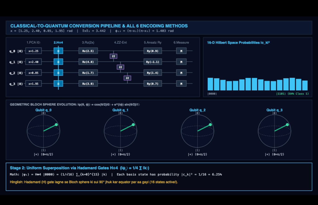
Visual mind map — how the paper's concepts, math & quantum stages connect
Click a branch of the map, or use the buttons below, to see how features, circuits, measurements and results connect.
Walk one candidate node pair (u, v) through all 6 quantum architectures side-by-side
Choose a scenario or move the sliders to follow one candidate pair through every stage: graph features, PCA and angles, the quantum state, the readout and the final probability p̂(u, v).
Results by network: persistence, quantum and classical
The five temporal networks from Paper 1. Pick one to compare the persistence rule (SeenBefore) with the best quantum and strongest classical configuration of each method, using the numbers reported in the paper.
Follow one pair of nodes from the graph to a prediction
Pick a stage, move the sliders, or click the first column to add a shared neighbour. Every number shown is computed by simulating the circuit.
Live circuit — exact amplitudes, Bloch vectors & export to Qiskit / OpenQASM
Data flow From raw events to a prediction, in eight steps
Circuits A four-qubit circuit, its 16 amplitudes and its Bloch spheres
Stage 1: dynamic stream S = {(u,v,t)} se 5 snapshots (G₁..G₄ → G₅)
Random walks DeepWalk, node2vec, Walklets and CTDNE on a small graph
1. DeepWalk vs Node2Vec biased walk mechanics
DeepWalk: unbiased random walks. From node v, each neighbour x ∈ Γ(v) is equally likely: P(x | v) = 1 / kv.
node2vec: second-order walks, where the next step depends on the previous node t as well as the current node v:
2. Walklets & Hadamard edge construction
Walklets: Explicitly skips k intermediate nodes in the random walk corpus to learn multi-scale representations zu = [zu(1) || zu(2) || zu(3)]. Scale k = 2 captures pure 2-hop triadic closure (A2), while scale k = 3 captures pure 3-hop paths (A3).
Hadamard product for pair embeddings (PQKELP): given node embeddings zu, zv ∈ ℝd, the pair vector is their element-wise product:
Taxonomy A map of link-prediction methods
| Method Family | Representative Architectures | Mathematical Mechanism | When to Apply & Limitations |
|---|---|---|---|
| 1. Local Heuristics (2-Hop) | Common neighbours (CN), Jaccard (JC), Adamic–Adar (AA), resource allocation (RA), preferential attachment (PA) | Counts common neighbours, each weighted by one over its degree: RA = ∑w ∈ Γ(u)∩Γ(v) 1kw. | Works well on dense social networks with strong triadic closure. Gives no signal when CN = 0. |
| 2. Global & Quasi-Local Heuristics (3-Hop & Path) | Shortest Path (SP), Local Path (LP), L3, CCLP, Katz Index, PageRank, SimRank | Degree-normalized 3-hop walks: L3 = ∑a,b 1√(kakb); Katz sums all path lengths: ∑ βlAl = (I − βA)−1 − I. | Needed on sparse bipartite, protein-interaction and citation graphs, where triangles are rare. |
| 3. Subgraph GNNs | SEAL (Zhang & Chen, NeurIPS 2018), NBFNet, Walk-Pooling GNN | Extracts the h-hop subgraph around (u, v), labels each node by its distances d(i,u) and d(i,v) (double-radius node labelling), and classifies the subgraph. | A strong static baseline, because it learns which structural patterns matter instead of fixing them by hand. |
| 4. Causal Temporal Random Walks | CTDNE (Nguyen et al., 2018) | Random walks that may only follow edges in time order: t1 ≤ t2 ≤ … ≤ tL. | Eliminates snapshots without neural overhead; preserves historical causality. |
| 5. Continuous-Time Memory Models | JODIE, DyRep, TGN (Rossi et al., 2020) | Keeps a memory su(t) for every node, updated by a GRU on each interaction (u, v, t, euv), with time encoded as φ(Δt) = cos(ωΔt + b). | The standard baseline for continuous-time event streams. A2QTGN builds its amplitude encoding on top of it. |
| 6. Dynamic Graph Mixers & Transformers | GraphMixer (ICLR 2023), DyGFormer (NeurIPS 2023) | GraphMixer summarises link history with small MLP-Mixers; DyGFormer splits a node's history into patches and attends over neighbour co-occurrence. | Among the strongest current models for continuous-time networks, and a natural target for future quantum feature maps. |
Select any network topology motif to compare classical heuristics vs. quantum link predictors live
Proposal A physics-informed variant (PI-QLP): graph diffusion, Hawkes processes and conservation constraints
The variational link predictors (PQCLP, QGCNLP, A2QTGN) are trained on a binary cross-entropy loss ℒBCE(θ) alone. On sparse snapshots this can overfit and mix up repeated edges with genuinely new ones. PI-QLP is a proposal, not a published method: it adds four physics-based penalties to the loss, with time derivatives computed by the parameter-shift rule.
Where & how PINN concepts apply across the 7 quantum link prediction papers
Instead of treating G1..G4 as unordered feature columns, encode time t in a gate RZ(ωt). The parameter-shift rule then gives ∂p̂θ/∂t exactly, and the loss penalises predictions that break heat diffusion on the Laplacian L(t) = D(t) − A(t).
Paper 1 found that repeated edges explain most of the measured accuracy. A Hawkes-process term separates the link intensity λuv(t) into a structural baseline μuvstruct, learned by the circuit for new edges ystrict, and an exponentially decaying memory for repeats.
In Paper 3 (QLPCN), computing U(t) = exp(−iAt) classically costs O(N3) and loses precision on large graphs. A shallow circuit |ψθ(t)⟩ trained on the Schrödinger residual could learn the walk on a changing adjacency matrix A(t) instead.
Requires the total predicted probability of new links at node u in G5 to match its degree growth Δku. This stops the model from inventing hubs where there is little data.
Related published literature: quantum PINNs (Q-PINNs) + physics-informed graph link prediction (GRAFF-LP / GRAND)
| Paper & Venue | Domain Circle | Core Mathematical Equation / Mechanism | How to Combine with Quantum Link Prediction | Links |
|---|---|---|---|---|
| 1. GRAFF-LP Di Francesco, Caso, Bucarelli & Silvestri (2024) arXiv:2402.14802 |
Physics-Inspired GNN for Link Prediction | Models GNN message passing as a physics gradient-flow PDE: ∂H(t)/∂t = −∇ EDirichlet(H(t)) |
Swap GRAFF-LP's linear edge decoder for a 4-qubit circuit or a projected quantum kernel, and keep its Dirichlet-energy loss. | |
| 2. Differentiable Quantum Circuits (DQC / Q-PINN) Kyriienko, Paine & Elfving (2021) Phys. Rev. A 103, 052416 |
Foundational Quantum PINN | Uses the parameter-shift rule on feature-encoded circuits to get exact derivatives ∂fθ(x,t)/∂t and minimise ℒPDE(θ). | Gives the differentiation rule needed to compute ∂p̂θ(e,t)/∂t for time-dependent link prediction. | |
| 3. Quantum PINNs on NISQ Systems Stefano Markidis (2022) Frontiers in Applied Mathematics and Statistics |
NISQ Quantum PINN Architecture | Combines several losses, ℒ = ℒdata + λPDEℒPDE + λBCℒBC, with RY/CNOT circuits. | Applies directly to PQCLP (Paper 4) and QGCNLP (Paper 6): add diffusion and degree-conservation terms to ℒBCE. | |
| 4. GRAND: Graph Neural Diffusion Chamberlain, Rowbottom, Gorinova, Webb, Rossi & Bronstein (2021) ICML 2021 |
Graph Heat Diffusion PDE | Treats graph propagation as continuous heat diffusion: ∂X(t)/∂t = div(G(X(t), t) ∇X(t)) |
Would replace the discrete GCN layers of QGCNLP (Paper 6) with continuous Laplacian diffusion weighted by quantum attention. | |
| 5. PDE-GCN Eliasof, Haber & Treister (2021) NeurIPS 2021 |
Hyperbolic Wave + Diffusion GCN | Moves between diffusion (∂u/∂t) and energy-conserving waves (∂²u/∂t² = −L u). | Sits between diffusive GNNs and the unitary quantum walk of Paper 3, U(t) = exp(−iAt), which behaves like a wave. | |
| 6. Quantum Physics-Informed Neural Networks Trahan, Loveland & Dent (2024) Entropy 26(8), 649 |
Q-PINN Optimizer & Depth Audit | Studies barren plateaus, optimiser convergence and expressibility in multi-layer quantum PINNs. | Consistent with Paper 1's set-up: shallow 4- to 6-qubit circuits with trust-region or hybrid optimisers. |
Watch how adding graph diffusion PDE & Hawkes ODE residuals eliminates overfitting & predicts future links across time t ∈ [t1, t5]
Change the penalty weights (λPDE, λHawkes, λflux) and the decay rate β. In the test window [t4, t5] the unconstrained circuit (red, dashed) drifts away from the expected trajectory, while PI-QLP (green) stays close to it. The curves are illustrative, not measured results.
Reference Formula sheet
Common neighbors (CN)
Counts shared 2-hop mutual friends.
Jaccard coefficient (JC)
Normalizes CN by total union of neighbors.
Adamic–Adar index (AA)
Penalizes high-degree common hubs logarithmically.
Resource allocation (RA)
Weights shared neighbors inversely by their full degree.
Preferential attachment (PA)
Captures rich-get-richer degree correlations.
Degree-normalized L3 (3-Hop)
Essential for protein-protein and bipartite networks.
Local path index (LP)
Combines 2-hop CN with ε-damped 3-hop extended paths.
Clustering coefficient LP (CCLP)
Sums the internal clustering coefficients Cw of shared neighbors.
Cannistraci–Hebb local community (CH-L2)
Ratio of internal local-community links to external links.
Click any mathematical symbol below to decode its meaning in plain English & Hinglish
Paper 1 · 2026 · this study Quantum Link Prediction in Dynamic Networks: Reproduction and Controlled Comparative Evaluation of Published Methods
Three major literature traps exposed
- Relabelled targets. Two of the methods report results against relabelled targets (yrel), which agree with the observed edges on only about half of all pairs. Against those targets the projected kernel won 59 of 60 comparisons.
- No leakage from preprocessing. Every scaler, PCA and angle rescaling is fitted on the training pairs and applied unchanged to the test pairs.
- Same inputs for both sides. A further comparator gives the classical models the same ten principal components the circuit receives. Against those inputs the circuit's features were significantly worse in 24 of 30 comparisons for one method and 28 of 30 for the other.
Key empirical findings & solutions
- The persistence rule. Predicting only previously seen pairs, with no parameters at all, reaches an AUC of 0.93–0.99 on four of the five networks. Most of the measured accuracy comes from repeated interactions.
- Same inputs for the classical side: a classical model trained on exactly the principal components the circuit receives separates the cost of compression, Δcompression, from the effect of the circuit, Δcircuit.
- COBYLA vs SPSA: with the published SPSA settings the PQCLP weights hardly moved from their starting values. With the same budget of evaluations, COBYLA raised the seed-1 test AUC to 0.62–0.80.
Reproduction pipeline code (Python / Qiskit)
# Strict Inductive Leak-Free Pipeline (Paper 1 Audit)
import numpy as np
from sklearn.preprocessing import StandardScaler
from sklearn.decomposition import PCA
from sklearn.ensemble import RandomForestClassifier
from qiskit.circuit.library import ZZFeatureMap, RealAmplitudes
from qiskit_algorithms.optimizers import COBYLA
from qiskit_machine_learning.algorithms import NeuralNetworkClassifier
from qiskit_machine_learning.circuit.library import QNNCircuit

# 1. Fit preprocessing strictly on train partition
scaler = StandardScaler()
X_tr_s = scaler.fit_transform(X_train)
X_te_s = scaler.transform(X_test)

pca = PCA(n_components=4)
X_tr_pca = pca.fit_transform(X_tr_s)
X_te_pca = pca.transform(X_te_s)

# Bounded non-linear scaling into (-pi, pi) for periodic gates
z_tr = np.pi * np.tanh(X_tr_pca)
z_te = np.pi * np.tanh(X_te_pca)

# 2. VQC Architecture: 4-Qubit ZZFeatureMap + RealAmplitudes
fmap = ZZFeatureMap(feature_dimension=4, reps=2, entanglement='linear')
ansatz = RealAmplitudes(num_qubits=4, reps=2, entanglement='ring')
qnn_qc = fmap.compose(ansatz)

qnn = QNNCircuit(num_qubits=4, feature_map=fmap, ansatz=ansatz)
vqc = NeuralNetworkClassifier(qnn, optimizer=COBYLA(maxiter=150), loss='binary_cross_entropy')
vqc.fit(z_tr, y_train)

# 3. Matched 4-PCA Classical Comparator
rf_matched = RandomForestClassifier(n_estimators=100, random_state=42)
rf_matched.fit(X_tr_pca, y_train)Test protocol leakage & target regime impact live (thakur et al., 2026)
Original paper PDF reader
Paper 2 · 2022 PQKLP: Projected Quantum Kernel based Link Prediction in Dynamic Networks
Theoretical innovation: solving fidelity concentration via 1-RDM projections
Full quantum state kernels k(x, x') = |⟨ψ(x)|ψ(x')⟩|² concentrate exponentially toward zero (2−n) as qubit count grows. PQKLP resolves this by evolving n = 11 qubits through a random rotation wall Uwall(r) + T = 10 Heisenberg Trotter steps (or 6 qubits with a ZZFeatureMap) and projecting onto single-qubit 1-RDMs via Pauli measurements: ρk(e) = Trj≠k[ρ(e)] = ½[I + ⟨Xk⟩X + ⟨Yk⟩Y + ⟨Zk⟩Z]. This produces a 33-dimensional (or 18-dimensional) classical expectation vector fed into 6 downstream classifiers.
The five networks, and how each circuit was run in Paper 1
Paper 1 uses five temporal networks, the ones shared by the snapshot-based methods: MIT (proximity), Radoslaw-email and Eu-core (e-mail), fb-forum (forum) and CollegeMsg (messaging). Partitioned into five snapshots, they reproduce all twenty-five published snapshot edge counts exactly.
| Model Family | Original Paper Circuit Formulation (PDF Spec) | Paper 1 Controlled Benchmark Formulation | Key Audit Finding in Paper 1 |
|---|---|---|---|
| PQKLP (2022) & PQKELP (2025) | n = 11 Qubits (PCA → 11D): H⊗11 → Ry(xi) → exp(−iπ3(XiXi+1 + YiYi+1 + ZiZi+1)) (1-layer Heisenberg/XY-Z evolution), measuring 33 single-qubit Pauli expectations. | 11 qubits in our reproduction. Ten principal components set the bond angles of a 10-step Trotter circuit (IsingXX, IsingYY, IsingZZ). The 33 Bloch values [⟨Xk⟩, ⟨Yk⟩, ⟨Zk⟩] go to classical classifiers, compared with the same classifiers on the same compressed features. | Projecting to single-qubit states avoids the concentration of full-state fidelity kernels. Even so, under the observed-edge target the classical counterpart was significantly better in 48 of 60 matched comparisons. |
| PQCLP (2024) | 4 or 8 qubits (local or global 16 features, combined 36, compressed by PCA): ZZ feature map followed by RealAmplitudes, trained with SPSA as published, or with COBYLA as a variant. | Splits the overall gap into two parts: Δtotal = Δcompression (16 → 4 features) + Δcircuit (4 classical features → 4-qubit circuit). | With the published SPSA step size the classifiers stayed close to their random initialisation; six of thirty mean AUCs were within 0.01 of 0.5. COBYLA, given the same budget, reached 0.62–0.80 on seed 1. |
| QGCNLP (2026) & A2QTGN (2026) | A two-block data re-uploading circuit (6n parameters) inside GCN message passing; 8-qubit amplitude encoding with an activity gate inside a TGN. | Message passing restricted to training edges (test edges removed from the normalised adjacency  = D̃−½ÃD̃−½), and node memory updated in time order only. | Prevents self-reinforcing test edge leakage during 2-hop neighborhood aggregation. |
PQKLP implementation code (Python / Qiskit)
import numpy as np
from qiskit.circuit.library import ZZFeatureMap
from qiskit.primitives import Estimator
from qiskit.quantum_info import SparsePauliOp
from sklearn.svm import SVC

# 1. 6-Qubit ZZFeatureMap (reps=2, linear entanglement)
fmap6 = ZZFeatureMap(feature_dimension=6, reps=2, entanglement='linear')

# 2. Build 18 Pauli Observables: X_k, Y_k, Z_k for all 6 qubits
pauli_ops = []
for k in range(6):
    for axis in ['X', 'Y', 'Z']:
        p_str = ['I'] * 6
        p_str[k] = axis
        pauli_ops.append(SparsePauliOp(''.join(p_str)))

# 3. 1-RDM Pauli Readout Function
estimator = Estimator()
def extract_1rdm_vector(z_vector_6d):
    bound_circ = fmap6.assign_parameters(z_vector_6d)
    job = estimator.run([bound_circ] * 18, pauli_ops)
    return job.result().values # 18-D vector

# 4. Train Classical Gaussian RBF-SVM on 18-D Quantum Projections
svm_clf = SVC(kernel='rbf', C=1.0)
svm_clf.fit(X_train_18d, y_train)Compare 6-Qubit 1-RDM projected kernel vs. global fidelity kernel
Original paper PDF reader
Paper 3 · 2023 Quantum Link Prediction in Complex Networks via Continuous-Time Quantum Walks
Physics insight: why continuous quantum walks outperform in PPI networks
Common-neighbour heuristics assume triadic closure. In bipartite and protein-interaction networks triangles are rare or impossible, so CN is often zero and gives no signal. QLPCN splits the walk into even orders, cos(At) = I − ½A²t² + …, and odd orders, sin(At) = At − ⅙A³t³ + …. In our reproduction the even branch scored higher on the social networks (Facebook, Hamsterster, Wiki-Vote) and the odd branch on HuRI, AS routes and Cora.
QLPCN continuous quantum walk code (Python / SciPy)
import numpy as np
from scipy.linalg import expm

# Direct Graph Adjacency Matrix A (No PCA, no heuristic indices!)
def qlpcn_transition_matrix(A_adj, t):
    # Hamiltonian simulation of Continuous-Time Quantum Walk: U(t) = exp(-i * A * t)
    U_t = expm(-1j * A_adj * t)
    # Quantum transition probability between nodes u and v: P_uv(t) = ||^2
    P_matrix = np.abs(U_t)**2
    return P_matrix

# In bipartite/PPI networks where triangles cannot form (CN = 0):
# Odd walks (3-hop paths A^3) naturally emerge from the sin(At) quantum interferometric amplitude!
t_opt = np.pi / 4
P_quantum = qlpcn_transition_matrix(A_graph, t_opt)
link_score = P_quantum[node_u, node_v] Tune continuous-time quantum walk evolution time t & even/Odd path weighting
Original paper PDF reader
Paper 4 · 2024 PQCLP: Parameterized Quantum Circuit based Link Prediction in Dynamic Networks
Theoretical innovation & SPSA vs. COBYLA optimizer audit
PQCLP trains a variational circuit end to end (ZZFeatureMap + RealAmplitudes, n = 4 or n = 8 qubits) and reads the link probability from qubit 0. In our reproduction the published SPSA step size (η = 0.001) moved no weight by more than 0.021 rad over 100 steps, so the classifier barely trained. With the same budget, COBYLA moved the weights by 1.4–2.6 rad and raised the seed-1 test AUC to 0.62–0.80.
PQCLP implementation code (Python / Qiskit)
from qiskit.circuit.library import ZZFeatureMap, RealAmplitudes
from qiskit_machine_learning.algorithms import NeuralNetworkClassifier
from qiskit_machine_learning.neural_networks import EstimatorQNN
from qiskit.quantum_info import SparsePauliOp
from qiskit_algorithms.optimizers import COBYLA

# 1. 4-Qubit Circuit: ZZFeatureMap Encoding + RealAmplitudes Ansatz
fmap4 = ZZFeatureMap(feature_dimension=4, reps=1, entanglement='linear')
ansatz4 = RealAmplitudes(num_qubits=4, reps=2, entanglement='ring')
qc = fmap4.compose(ansatz4)

# 2. Computational Basis Readout on Qubit 0:
# P(q0=1) = 0.5 * (1 - )
obs_z0 = SparsePauliOp.from_list([('IIIZ', 1.0)])

qnn = EstimatorQNN(
    circuit=qc,
    input_params=fmap4.parameters,
    weight_params=ansatz4.parameters,
    observables=[obs_z0]
)

# 3. Train End-to-End VQC via COBYLA with Binary Cross-Entropy Loss
opt = COBYLA(maxiter=120)
vqc_clf = NeuralNetworkClassifier(neural_network=qnn, optimizer=opt, loss='binary_cross_entropy')
vqc_clf.fit(X_train_pca4, y_train) Explore 4-Qubit end-to-end VQC depth vs. qubit-0 readout
Original paper PDF reader
Paper 5 · 2025 PQKELP: Projected Quantum Kernel Embedding based Link Prediction via Random Walks
Theoretical motivation: overcoming triadic sparsity with multi-scale Walklets
In real dynamic graphs, over 90% of candidate node pairs have zero common neighbors (CN = 0). PQKELP overcomes this by learning 128-D Node2Vec, DeepWalk, and multi-scale Walklets (k ∈ {1..4}) across G1..G4, forming edge Hadamard products zu ⊙ zv ∈ ℝ1536, compressing via PCA to ℝ10, and projecting through an 11-qubit Heisenberg Trotter 1-RDM circuit into ℝ33 (or 5-qubit ZZFeatureMap into ℝ15).
PQKELP implementation code (Python / Qiskit)
from node2vec import Node2Vec
from qiskit.circuit.library import ZZFeatureMap
from sklearn.decomposition import PCA
from sklearn.svm import SVC
import numpy as np

# 1. Generate Multi-Scale Random Walk Embeddings (e.g. Node2Vec p=1.0, q=0.5)
n2v = Node2Vec(graph_G4, dimensions=64, walk_length=20, num_walks=10, p=1.0, q=0.5)
model = n2v.fit(window=5, min_count=1)

# 2. Hadamard Edge Embedding: h(u,v) = z_u * z_v
edge_feats = [model.wv[str(u)] * model.wv[str(v)] for (u, v) in edges]

# 3. PCA to 5 Dimensions + Bounded tanh scaling into (-pi, pi)
pca5 = PCA(n_components=5)
X_pca5 = pca5.fit_transform(edge_feats)
z_5d = np.pi * np.tanh(X_pca5)

# 4. 5-Qubit ZZ Feature Map with 15-D Pauli Bloch Readout
fmap5 = ZZFeatureMap(feature_dimension=5, reps=2, entanglement='linear')
# Measure , ,  for each of the 5 qubits -> produces 15D vector
X_bloch_15d = extract_pauli_bloch_15d(fmap5, z_5d)

# 5. Train SVM Classifier
svm_clf = SVC(kernel='rbf', C=1.0).fit(X_bloch_15d, y_train) Inspect π·tanh(z) non-linear squashing & 15-D full Bloch vector
Original paper PDF reader
Paper 6 · 2026 QGCNLP: Quantum Graph Convolutional Network for Link Prediction
Theoretical innovation: node-level data re-uploading quantum GCN (O(N) vs. O(N2))
QGCNLP embeds a 2-block Data Re-Uploading quantum circuit (n = 4 or 8 qubits, all-pairs CNOT entanglement Call, and 6n trainable RYRXRZ rotations) directly inside each node-level GCN message-passing layer (O(N) circuit evaluations per layer instead of O(N2) edge circuits). Residual LayerNorm fusion H(l+1) = LayerNorm(WefQ + h(l)) guarantees stability, while the quantum layer is differentiated via the analytical Parameter-Shift Rule: ∂⟨Z⟩/∂θj = ½[⟨Z(θj + π/2)⟩ − ⟨Z(θj − π/2)⟩].
QGCNLP hybrid implementation code (PyG + PennyLane)
import torch
import torch.nn as nn
from torch_geometric.nn import GCNConv
import pennylane as qml

# 1. 4-Qubit PennyLane Device with Analytical Parameter-Shift
dev = qml.device("default.qubit", wires=4)

@qml.qnode(dev, diff_method="parameter-shift")
def qgcn_quantum_circuit(inputs, weights):
    for i in range(4): qml.RY(inputs[i], wires=i)
    for i in range(4):
        qml.CNOT(wires=[i, (i + 1) % 4])
        qml.RY(weights[i], wires=i)
    return [qml.expval(qml.PauliZ(i)) for i in range(4)]

# 2. Hybrid Classical GCN + Quantum Edge Classifier
class QGCNLP(nn.Module):
    def __init__(self, in_dim, hidden_dim):
        super().__init__()
        self.gcn1 = GCNConv(in_dim, hidden_dim)
        self.gcn2 = GCNConv(hidden_dim, 16)
        self.proj = nn.Linear(32, 4) # [h_u || h_v] -> 4 angles
        self.q_weights = nn.Parameter(torch.randn(4))
        self.out_head = nn.Linear(4, 1)

    def forward(self, x, edge_index, edge_pairs):
        h = torch.relu(self.gcn1(x, edge_index))
        h = self.gcn2(h, edge_index)
        u_emb = h[edge_pairs[:, 0]]
        v_emb = h[edge_pairs[:, 1]]
        q_in = torch.tanh(self.proj(torch.cat([u_emb, v_emb], dim=-1))) * 3.14159

        # Pass through quantum node
        q_out = torch.stack([torch.tensor(qgcn_quantum_circuit(q_in[i], self.q_weights)) for i in range(len(q_in))])
return torch.sigmoid(self.out_head(q_out))Simulate hybrid GCN message-passing + parameter-shift gradient
Original paper PDF reader
Paper 7 · 2026 A2QTGN: Adaptive Amplitude Quantum-Integrated Temporal Graph Network
Theoretical innovation: conditional activity-gated 8-Qubit amplitude encoding
A2QTGN eliminates snapshot quantization by integrating a continuous-time Temporal Graph Network (64-D memory mu,tprev) with an Activity Gate αu,t = σ(β‖xu,t − xu,tprev‖2). Quiescent nodes (αu,t ≤ τ) reuse their cached quantum state; active nodes (αu,t > τ) encode all 256 features into just 8 qubits (28 = 256 basis states, depth 1,011 + linear CNOT chain; or 16 features into 4 qubits in compact mode) and fuse ⟨Z0..Z7⟩ ∈ ℝ8 with TGN memory.
A2QTGN implementation code (PennyLane / PyTorch)
import torch
import numpy as np
import pennylane as qml

# 4-Qubit Device: Encodes 2^4 = 16 continuous features into amplitudes!
dev4 = qml.device("default.qubit", wires=4)

@qml.qnode(dev4)
def a2qtgn_circuit(amplitudes_16d, vqc_weights):
    # Möttönen Amplitude State Preparation
    # |psi> = sum_{j=0}^15 alpha_j |j> where sum |alpha_j|^2 = 1
    qml.AmplitudeEmbedding(features=amplitudes_16d, wires=range(4), normalize=True)

    # Entangling Variational Quantum Layers
    for i in range(4):
        qml.RY(vqc_weights[i], wires=i)
        qml.CNOT(wires=[i, (i + 1) % 4])

    return [qml.expval(qml.PauliZ(i)) for i in range(4)]

# Pipeline:
# 1. Continuous TGN updates memory state: s_u(t) = GRU(s_u(t-), msg_u(t))
# 2. Extract 16D edge embedding h_uv(t) with temporal graph attention
# 3. L2 normalize into state amplitudes and evaluate VQC:
alpha_norm = raw_16d / np.linalg.norm(raw_16d)
vqc_readout = a2qtgn_circuit(alpha_norm, vqc_theta)Compare adaptive amplitude compression (2^q features in q qubits) vs. angle encoding
Original paper PDF reader
Visual maths The matrix algebra behind the methods: products, tensor products, partial traces and interference
How matrix multiplication counts walks: click any cell (u, v) in A, A2 (2-Hop CN), or A3 (3-Hop L3)
Why is (A2)uv = ∑w AuwAwv the number of common neighbours, and why does (A3)uv count 3-hop paths? Click a cell (u, v) in the matrices below, or toggle edges in the graph.
See the exact 4×4 unitary matrix U multiply the 4×1 statevector |ψ⟩ gate-by-gate
A 16×16 matrix is too big to read, so this uses two qubits (a 4-dimensional state). You can see every entry of H⊗H, RY(z0)⊗RY(z1), the CNOT and the ZZ gate.
Why PQKLP (2022) & PQKELP (2025) use 1-RDM partial trace ρk = trj≠k[|ψ⟩⟨ψ|] instead of global fidelity
Move the entanglement strength αent and the qubit count q. Tracing out the other qubits turns a pure state into a mixed 2×2 density matrix ρ0, and the projected kernel stays informative while the full fidelity kernel collapses.
Why U(t) = exp(−iAt) = cos(At) − i sin(At) splits social (2-Hop) vs. bipartite (3-Hop) networks
Taylor expansion shows cos(At) = I − t22!A2 + t44!A4 (Even walks = Triadic Closure) while sin(At) = tA − t33!A3 (odd walks: 3-hop, L3-like)
How ZZFeatureMap warps 2D PCA space (z1, z2) via cos((π−z1)(π−z2))
Compare a linear decision boundary with the curved contours of the ZZ term Φ12(z) = (π − z1)(π − z2).
Foundations Graph basics for link prediction, with a worked example
1. The 5 fundamental graph quantities & matrix powers (A, A2, A3)
For undirected graphs without self-loops, A is symmetric (A = A⊤) with zeros on the diagonal (Auu = 0).
(Ak)uv counts exact k-step walks between u and v! (A2)uv is 2-hop Common Neighbors (triadic closure); (A3)uv is 3-hop paths (bipartite / PPI closure).
High-degree hubs (ku ≫ 1) act as noisy bridges, which is why Adamic–Adar (1/log kw) and Resource Allocation (1/kw) penalize high-degree common neighbors.
Measures what fraction of node u's neighbors are also friends with each other. High Cu > 0.25 indicates social triadic closure; Cu = 0 indicates bipartite / triangle-free structure.
2. The 5 core research pillars of social network analysis (classical vs. quantum paradigm)
| SNA Research Pillar | Core Mathematical Question | Classical SNA Algorithms | Quantum SNA Algorithms & Advantage |
|---|---|---|---|
| 1. Node Centrality & Influence | Which actors are the most influential hubs or bridges in G? | Degree ku, Betweenness, Closeness, Eigenvector Centrality, PageRank | Quantum PageRank and CTQW centrality (Szegedy walks, or where a continuous-time walk tends to localise) |
| 2. Community Detection | Which densely connected clusters or modular groups exist in G? | Louvain Modularity, Girvan–Newman, Spectral Clustering (L = D − A), Infomap | QAOA for modularity (HC = −½∑ BuvZuZv) and quantum-walk trapping |
| 3. Link Prediction (Primary Focus) | Which unobserved or future edges (u, v) will form in GT? | CN, JC, AA, RA, PA, Katz, LP, L3, DeepWalk, Node2Vec, Walklets, GCN, TGN | PQKLP (1-RDM Kernel), QLPCN (CTQW Even/Odd), PQCLP (VQC), PQKELP (Walk Kernel), QGCNLP, A2QTGN |
| 4. Information Diffusion & Cascades | How fast do rumors, epidemics, or signals spread across G? | SIR / SIS Epidemic Models, Independent Cascade, Linear Threshold | Ballistic spreading of quantum walks (width grows as σ(t) ∝ t, against √t for a classical random walk) |
| 5. Dynamic Network Evolution | How do graph motifs and temporal interactions evolve over time? | Snapshot Decay e−λ(T−t), CTDNE, Temporal Point Processes | A2QTGN Activity-Gated Quantum Memory & Temporal Snapshot Feature Encodings |
Step-by-step numerical trace: candidate edge e = (u, v) across all 5 pipeline stages
Pick a candidate link from the worked example, or move the snapshot sliders, and every matrix, z-score, principal component, gate angle and probability updates.
Static graphs Static link prediction without leakage, community features and QAOA modularity
1. Static graph link prediction: the zero-leakage edge-masking protocol (E = Eobs ∪ Etest)
Hide 20% of the true edges at random as positive test targets Etest, keeping the graph connected, and build the observed adjacency matrix Aobs from Eobs only.
If Etest stays in A while CN, AA, Katz or a GCN are computed, a test pair (u,v) has shortest path 1 and raises its own neighbours' degrees, so the label y = 1 leaks into the features.
Sample the same number of non-edges Eneg ⊂ (V×V) ∖ E. Fit the scaler (μ, σ) and the PCA matrix Wq on training pairs only, then encode into the q-qubit circuit.
2. Community-aware classical link prediction indices & quantum QAOA max-modularity Hamiltonian
Modularity matrix Buv & quality Q
Measures how many more edges a pair has than a random graph with the same degrees would give. Pairs with Buv > 0 and cu = cv are likely to link inside their community.
Community-boosted common neighbors (SH-CN & WIC)
Gives double weight to common neighbours w in the same community as both endpoints (cu = cv = cw), and compares shared neighbours inside and across clusters.
Local community paradigm (CAR & CH-L2)
Without community labels, CAR and CH-L2 count the links among the shared neighbours themselves (dint(w)) against their links outside (dext(w)).
Ising modularity Hamiltonian & QAOA ansatz
Minimising ⟨ψ|HC|ψ⟩ pushes the spins ⟨Zu⟩, ⟨Zv⟩ of nodes in the same community to the same sign. The correlation ⟨ZuZv⟩ can then serve as a score for links inside a community.
Live static graph edge-masking & QAOA max-modularity spin partitioning
Pick a candidate pair, or change the QAOA cost angle γ and mixer angle β, to see how the spin correlations ⟨ZuZv⟩ separate the communities and score the hidden test links.
Design decisions Why not feed the whole adjacency matrix? Choosing features, techniques and optimisers
Q1. Why can't we feed the full N × N adjacency matrix directly into a variational quantum circuit? (The 4 physical walls)
Encoding one feature per qubit for every pair of a 1,000-node graph would need q = N(N−1)/2 ≈ 5×10⁵ qubits. Today's devices have roughly 100 to 1,000 noisy qubits.
For deep random circuits on q = 50 qubits, gradient variance shrinks like 2−50 ≈ 10−15, far below shot noise. Compressing to a few qubits with PCA keeps gradients measurable.
All-to-all ZZ coupling on q qubits needs q(q−1)/2 two-qubit gates per layer. A ring on 4 qubits needs only 4 CNOTs; at 100 qubits, thousands of noisy CNOTs drive the state towards the maximally mixed state I/2q.
Raw features such as PA = kukv can range from 0 to 10,000. Rotations are periodic, so without scaling, PCA and π tanh(·), PA = 1 and PA = 1 + 2π land on exactly the same state.
Q2 & Q3. Where to apply local vs. quasi-local vs. global features — and why papers use different features on the same dataset
| Feature Family | Exact Indices & Walk Depth | When & Where to Apply (Network Physics) | Why Different Papers Use Different Subsets on radoslaw-email / email-Eu-core |
|---|---|---|---|
| 1. Local 2-Hop Heuristics | CN, JC, AA, RA, PA, CCLP(Walk length l = 2, complexity O(⟨k⟩2)) |
Dense social and e-mail networks (clustering C > 0.25), where friends of friends quickly close triangles. | PQCLP's local feature set (4×4 = 16) keeps only 2-hop signals, to test whether a 4-qubit circuit can learn triadic closure on its own. |
| 2. Quasi-Local 3-Hop Paths | LP (Local Path), L3 (Degree-Normalized 3-Hop)(Walk length l = 3, complexity O(⟨k⟩3)) |
Bipartite, protein-interaction and user–item graphs, where triangles cannot form (A2uv = 0 between the two sides) and new links close 4-cycles through 3-hop paths. Also sparse social graphs where CN is often zero. | QLPCN (2023) reports that odd walks, sin(At), do better on protein networks. PQCLP's global and combined sets add LP and L3 to capture the 3-hop paths CN misses. |
| 3. Global All-Paths Indices | SP (Shortest Path), Katz, RWR, SimRank(Walk length l → ∞, complexity O(N3)) |
Sparse infrastructure, citation and cold-start networks, where candidate pairs are four or more hops apart and both CN and L3 are zero. | PQKLP (2022) combines five local indices (CN, JC, AA, RA, PA) with one global index (SP) across the four history snapshots, 6×4 = 24 features, before PCA. |
| 4. Learned Walk / GNN / Temporal Memory | PQKELP (Random Walk Hadamard), QGCNLP (Variational GCN), A2QTGN (Event Memory) |
Multi-scale and continuous-time streams, where hand-built features miss longer-range context or bursts inside a snapshot. | The papers try richer representations in turn on the same benchmark networks: hand-built features (PQKLP), an end-to-end circuit (PQCLP), random-walk embeddings (PQKELP), a quantum GCN (QGCNLP) and event memory (A2QTGN). |
Q4. How do we know which link prediction technique is best for any dataset?
Describe your dataset with the four questions below to get a suggested feature set and architecture.
How quantum circuits train: parameter-shift rule vs. COBYLA simplex vs. SPSA perturbation
Why backpropagation does not pass through a measurement, how the parameter-shift rule gives exact gradients, and what happened with COBYLA and SPSA in our reproduction.
Pauli rotations have generator eigenvalues ±½, so shifting θk by ±π/2 gives the exact derivative, with no finite-difference error.
Perturbs all P parameters at once along a random direction Δt ∈ {±1}P. With the small published step size the weights barely moved, and the classifiers scored close to 0.5.
Keeps a simplex of P+1 points inside a shrinking trust region ρt. With the same evaluation budget as SPSA it reduced the training loss by 0.08–0.23 and reached a seed-1 test AUC of 0.62–0.80.
Further reading on quantum link prediction and quantum graph learning
Each entry links to its source (arXiv, OpenReview, APS, Elsevier, IEEE Xplore, MDPI, CEUR-WS, or a local PDF). Filter by category or search by keyword, author or circuit type.
QGraphGAN: quantum graph softmax for adversarial link prediction via BFS-tree variational circuits
Replaces each branch scorer in GraphGAN's BFS-tree generator with a variational quantum circuit, to isolate what the quantum part contributes to adversarial link prediction.
On the complexity of quantum link prediction in complex networks
Works out the query complexity, state-preparation cost and shot counts needed for quantum-walk link prediction, and when a polynomial speed-up can hold.
QSearchNet: A quantum walk search framework for link prediction
A quantum-walk search framework between local common-neighbour heuristics and global Katz-style path counts, using interference to move between the two.
Community-aware quantum link prediction in complex networks with inter-community information
Adds community structure and inter-community bridge weights to quantum-walk link prediction, and reports better rankings on modular social and biological networks.
Link prediction with continuous-time classical and quantum walks
Compares classical diffusion exp(−Lt) with continuous-time quantum walks exp(−iAt) and exp(−iLt) for link prediction on several network types.
GCQW: A quantum walk model for predicting missing links of complex networks
Uses discrete-time, Grover-coined quantum walks to accumulate multi-hop amplitudes between unconnected pairs.
Towards quantum graph neural networks: an ego-graph learning approach (egoQGNN)
Splits large graphs into k-hop ego networks small enough for near-term circuits to do message passing, for link prediction and node classification.
Inductive graph representation learning with quantum graph neural networks
An inductive, neighbourhood-sampling quantum graph network, similar in spirit to GraphSAGE, that can handle unseen nodes and evolving graphs.
A critical review of quantum graph neural networks
A critical review of quantum graph convolution and message passing: encoding bottlenecks, barren plateaus, and whether classical baselines are compared fairly.
Quantum negative sampling strategy for knowledge graph embedding & link prediction
Uses superposition to choose informative negative samples for knowledge-graph completion and link prediction.
Incorporating content-based features into quantum knowledge graph embeddings for link prediction
Combines text embeddings with parameterised circuits for relational link prediction in knowledge graphs.
Power of data in quantum machine learning (introduces projected quantum kernels & yrel)
Introduced the projected quantum kernel, built from single-qubit reduced states ρk = Trj≠k(|ψ⟩⟨ψ|), together with a Trotterised Heisenberg circuit and the geometric difference Ω = KC−1/2KQKC−1/2 for asking when a quantum kernel can help. PQKLP (2022) and PQKELP (2025) build on it.
Information-theoretic bounds on quantum advantage in machine learning
Shows why inner products over the full Hilbert space concentrate exponentially, and gives sample-complexity bounds for classical shadows and reduced-state projections.
Quantum graph neural networks (foundational QGNN & QGCNN formulation)
Early quantum graph neural networks and quantum graph convolutions, alternating graph-coupled Ising Hamiltonians with single-node rotations.
Quantum link prediction in dynamic networks: reproduction and controlled comparative evaluation of published methods
Re-implements five published quantum link-prediction methods and a quantum-walk reference under one leak-free snapshot protocol on five temporal networks. Compares each with matched classical counterparts using paired tests, and adds controls for repeated edges and relabelled targets.
PQKLP: projected quantum kernel based link prediction in dynamic networks
Compresses the snapshot features to 10 principal components, runs a 10-step Trotter circuit on 11 qubits, and gives the 33 single-qubit Pauli values to six classical classifiers.
QLPCN: quantum link prediction in complex networks via continuous-time quantum walks
Runs an ancilla-controlled continuous-time quantum walk e∓iAtw on the adjacency matrix to separate even path lengths (cos(Atw), typical of social networks) from odd ones (sin(Atw), typical of protein networks).
PQCLP: parameterized quantum circuit based link prediction in dynamic networks
Trains a 4-qubit (local or global features) or 8-qubit (combined) variational classifier, a 2-repetition ZZFeatureMap followed by a 2-repetition RealAmplitudes, read out on qubit 0.
PQKELP: projected quantum kernel embedding based link prediction via random walks
Combines node2vec, DeepWalk and multi-scale Walklets embeddings per pair with Hadamard products, compresses them to 10 principal components, and projects them through an 11-qubit Trotter circuit to 33 Pauli values.
QGCNLP: hybrid quantum–Classical graph convolutional network based link prediction
Places a two-block data re-uploading circuit (n = 4 or 8 qubits) inside each GCN layer, one call per node (O(N)), with residual LayerNorm and a cosine-similarity decoder.
A2QTGN: adaptive amplitude quantum-integrated temporal graph network for dynamic link prediction
Gates each event by node activity (αu,t > τ), amplitude-encodes a 256-dimensional vector into 8 qubits, and combines it with TGN memory to predict links in an event stream.
Upload Your SNA Dataset — Full Network Story, Topology Audit & Quantum Link Prediction Diagnosis
Drop any Social Network Analysis (SNA) dataset below (edge list u v [timestamp/weight] in .csv, .tsv, .txt, .edges, .gml, .json, or .gz) or paste raw edges. The studio immediately profiles your network's scale, connected components, hubs, triadic closure vs. 3-hop bipartite structure, assortativity, and temporal persistence, explains what the graph looks like in plain language, recommends which of the 7 Quantum Link Prediction architectures fits best, and predicts the top missing links using exact quantum statevector simulation.
source target [timestamp]), JSON ({"edges":[[u,v],...]} or {"links":[{"source":u,"target":v}]}), GML (edge [ source u target v ]), or gzipped .gz files. Everything runs 100% locally in your browser.
u v or u,v,timestamp):
1. What Your Uploaded SNA Dataset Tells Us (Automated Executive Briefing)
2. Network Topology & Top Predicted Links
Nodes colored by structural role (● Hubs, ● Core/Bridge, ● Periphery). Dashed emerald arcs show the highest-probability missing links predicted by the quantum kernel.
3. Degree Distribution P(k) & Motif Profile
Left: node degree histogram (detects scale-free hubs vs. uniform random degree). Right: normalized strength of 2-hop triads (A2), 3-hop bipartite paths (L3), and hub attachment (PA).
4. Quantum Link Prediction Architecture Suitability Matrix (Tailored to Your Graph)
Evaluates how each of the 7 landmark papers behaves on your uploaded network's exact node count, clustering coefficient, 2-hop vs. 3-hop balance, and temporal persistence:
5. Top 10 Most Influential Nodes (Centrality & Structural Role)
Ranked by degree centrality, local clustering coefficient Ci, 2-hop neighborhood reach, and eigenvector/PageRank hub score.
6. Top 10 Predicted Missing Links (u, v) (Classical + Exact Quantum)
Highest-scoring unconnected node pairs in your graph across Common Neighbors (CN), Adamic-Adar (AA), 3-Hop (L3), 4-Qubit Projected Quantum Kernel (PQK), 4-Qubit VQC, and Quantum Walk (CTQW).